


Correlation the Number of the Students’ College Applications and Consumption of Caffeine
Introduction and statement of intent:
Students are exposed to a lot of stress during the college admissions process. These increased stress levels come with some negative consequences like the increase in consumption of caffeine. The objective of this academic project is to find out whether the number of colleges high school seniors are applying to increases the consumption of stimulant substances like caffeine. I will explore the relationship between the amount of college applications and the daily consumption of coffee within the population of high school seniors. I selected this topic because, as a senior, the massive number of college applications need to submit has affected noticeably the quantity of caffeine I personally consume. On the basis of this study I will try to know if this is a rule that can be applied in a more general basis or not.
If you need assistance with writing your essay, our professional essay writing service is here to help!
In order to collect the primary data, I used direct interview method. For accurate and reliable information, the data was collected from 50 seniors in different schools in different countries. I collected information regarding different possible variables in order to be able to decide which one would give me the most accurate information for the exploration. Finally, I decided to stick to the data related to the number of cups of coffee that a student takes daily and the number of colleges that student is applying to. I will be using in order to get to a conclusion, my data, several mathematical calculations to see if there is a relation between the two variables and use of scatter diagram for better presentation and understanding of the topic.
Initially, to find out about the relationship between my two variables (number of college applications and coffee consumption), my data will be plotted on an scatter-diagram, as well as find the Pearson’s correlation coefficient (r). I will effectuate a rather a chi-squared test or the regression equation depending on the value of r that obtain to make some predictions. This, will allow me to determine the liability of the regression line to make predictions about my data, and if the variables are independent or not by testing the null hypothesis in the chi-squared test if necessary.
Correlation Analysis:
Correlation is used to define the linear relationship between two continuous variables. A correlation could be positive, (both variables move in the same direction), or negative (when one variable’s value increases, the other variables’ values decrease). Correlation can also be zero (variables are unrelated). The strength/qualitatively and direction of the linear relationship between two or more variables.
Correlation allows me to clearly and easily see if there is a relationship between variables. This relationship can then be displayed in a graphical form. It also gives a precise quantitative value indicating the degree of relationship existing between the two variables and it measures the direction and the relationship between the two variables.
Assumptions:
There are some vital assumptions are required to establish correlation between two variables. These assumptions are:
- Both variables (Number of Applications and Number of Cups of Coffee a day (8 oz.)) is normally distributed.
- Second assumption includes linearity. Linearity assumes that there is a straight-line relationship
between each of the two variables and on other hand.
Mathematical investigation:
Data:
| Number of
applications |
Number of cups
of coffee a day (8 oz.) |
Number of applications | Number of cups
of coffee a day (8 oz.) |
||
| 1 | 10 | 4 | 26 | 11 | 3 |
| 2 | 15 | 5 | 27 | 6 | 2 |
| 3 | 3 | 0 | 28 | 16 | 7 |
| 4 | 11 | 6 | 29 | 20 | 8 |
| 5 | 11 | 5 | 30 | 11 | 3 |
| 6 | 19 | 9 | 31 | 18 | 5 |
| 7 | 6 | 2 | 32 | 9 | 3 |
| 8 | 12 | 4 | 33 | 16 | 3 |
| 9 | 5 | 1 | 34 | 2 | 0 |
| 10 | 17 | 7 | 35 | 10 | 3 |
| 11 | 21 | 8 | 36 | 9 | 2 |
| 12 | 10 | 1 | 37 | 6 | 1 |
| 13 | 8 | 3 | 38 | 4 | 0 |
| 14 | 6 | 2 | 39 | 13 | 2 |
| 15 | 7 | 2 | 40 | 21 | 7 |
| 16 | 10 | 0 | 41 | 14 | 3 |
| 17 | 14 | 4 | 42 | 2 | 1 |
| 18 | 13 | 3 | 43 | 10 | 3 |
| 19 | 1 | 0 | 44 | 7 | 2 |
| 20 | 12 | 3 | 45 | 15 | 6 |
| 21 | 15 | 6 | 46 | 4 | 1 |
| 22 | 18 | 9 | 47 | 12 | 4 |
| 23 | 4 | 1 | 48 | 1 | 0 |
| 24 | 7 | 2 | 49 | 15 | 6 |
| 25 | 24 | 8 | 50 | 11 | 2 |
Mathematical Process to get the Correlation Coefficient (r):
Step 1: Making a chart with data for two variables, labelling the variables (x) and (y), and add three more columns labelled (XY), (X2), and (Y2).
Step 2: Complete the chart using basic multiplication of the variable values.
Computation of Karl Pearson’s Coefficient of correlation: (Direct Method)
Step 3: After multiplied all the values to complete the chart, add up all of the columns from top to bottom.
Step 4: Use the following formula to find the Pearson correlation coefficient value.
Pearson’s Correlation Coefficient (r):
r=n xy–(x*y)nx2–(x)2* ny2–(y)2
r=502,496–(542*172)50 7,444–(542)2* 50(916)–(172)2
r=1,24,800–93,2243,72,200– 2,93,764* 45,800–29,584
r=31,57678,436* 16,216
r=31,576280.06427* 127.3420 r=31,57635,663.9442 =0.89
Step: 6 Solving with the formula above by plugging in all the correct values, the result is thecoefficient value.
If the value is a negative number, then there is a negative correlation, and if the value is a positive number, then there is a positive correlation.
Pearson’s Correlation coefficient
| Sr. No. | X | Y | (X–X̅) | (X–X)2̅ | (Y–Y̅) | (Y–Y)2̅ | X–X̅(Y–Y̅) |
| 1 | 10 | 4 | -0.84 | 0.71 | 0.56 | 0.31 | -0.47 |
| 2 | 15 | 5 | 4.16 | 17.31 | 1.56 | 2.43 | 6.49 |
| 3 | 3 | 0 | -7.84 | 61.47 | -3.4 | 11.83 | 26.97 |
| 4 | 11 | 6 | 0.16 | 0.03 | 2.56 | 6.55 | 0.41 |
| 5 | 11 | 5 | 0.16 | 0.03 | 1.56 | 2.43 | 0.25 |
| 6 | 19 | 9 | 8.16 | 66.59 | 5.56 | 30.91 | 45.37 |
| 7 | 6 | 2 | -4.84 | 23.43 | -1.4 | 2.07 | 6.97 |
| 8 | 12 | 4 | 1.16 | 1.35 | 0.56 | 0.31 | 0.65 |
| 9 | 5 | 1 | -5.84 | 34.11 | -2.4 | 5.95 | 14.25 |
| 10 | 17 | 7 | 6.16 | 37.95 | 3.56 | 12.67 | 21.93 |
| 11 | 21 | 8 | 10.16 | 103.23 | 4.56 | 20.79 | 46.33 |
| 12 | 10 | 1 | -0.84 | 0.71 | -2.4 | 5.95 | 2.05 |
| 13 | 8 | 3 | -2.84 | 8.07 | -0.4 | 0.19 | 1.25 |
| 14 | 6 | 2 | -4.84 | 23.43 | -1.4 | 2.07 | 6.97 |
| 15 | 7 | 2 | -3.84 | 14.75 | -1.4 | 2.07 | 5.53 |
| 16 | 10 | 0 | -0.84 | 0.71 | -3.4 | 11.83 | 2.89 |
| 17 | 14 | 4 | 3.16 | 9.99 | 0.56 | 0.31 | 1.77 |
| 18 | 13 | 3 | 2.16 | 4.67 | -0.4 | 0.19 | -0.95 |
| 19 | 1 | 0 | -9.84 | 96.83 | -3.4 | 11.83 | 33.85 |
| 20 | 12 | 3 | 1.16 | 1.35 | -0.4 | 0.19 | -0.51 |
| 21 | 15 | 6 | 4.16 | 17.31 | 2.56 | 6.55 | 10.65 |
| 22 | 18 | 9 | 7.16 | 51.27 | 5.56 | 30.91 | 39.81 |
| 23 | 4 | 1 | -6.84 | 46.79 | -2.4 | 5.95 | 16.69 |
| 24 | 7 | 2 | -3.84 | 14.75 | -1.4 | 2.07 | 5.53 |
| 25 | 24 | 8 | 13.16 | 173.19 | 4.56 | 20.79 | 60.01 |
| 26 | 11 | 3 | 0.16 | 0.03 | -0.4 | 0.19 | -0.07 |
| 27 | 6 | 2 | -4.84 | 23.43 | -1.4 | 2.07 | 6.97 |
| 28 | 16 | 7 | 5.16 | 26.63 | 3.56 | 12.67 | 18.37 |
| 29 | 20 | 8 | 9.16 | 83.91 | 4.56 | 20.79 | 41.77 |
| 30 | 11 | 3 | 0.16 | 0.03 | -0.4 | 0.19 | -0.07 |
| 31 | 18 | 5 | 7.16 | 51.27 | 1.56 | 2.43 | 11.17 |
| 32 | 9 | 3 | -1.84 | 3.39 | -0.4 | 0.19 | 0.81 |
| 33 | 16 | 3 | 5.16 | 26.63 | -0.4 | 0.19 | -2.27 |
| 34 | 2 | 0 | -8.84 | 78.15 | -3.4 | 11.83 | 30.41 |
| 35 | 10 | 3 | -0.84 | 0.71 | -0.4 | 0.19 | 0.37 |
| 36 | 9 | 2 | -1.84 | 3.39 | -1.4 | 2.07 | 2.65 |
| 37 | 6 | 1 | -4.84 | 23.43 | -2.4 | 5.95 | 11.81 |
| 38 | 4 | 0 | -6.84 | 46.79 | -3.4 | 11.83 | 23.53 |
| 39 | 13 | 2 | 2.16 | 4.67 | -1.4 | 2.07 | -3.11 |
| 40 | 21 | 7 | 10.16 | 103.23 | 3.56 | 12.67 | 36.17 |
| 41 | 14 | 3 | 3.16 | 9.99 | -0.4 | 0.19 | -1.39 |
| 42 | 2 | 1 | -8.84 | 78.15 | -2.4 | 5.95 | 21.57 |
| 43 | 10 | 3 | -0.84 | 0.71 | -0.4 | 0.19 | 0.37 |
| 44 | 7 | 2 | -3.84 | 14.75 | -1.4 | 2.07 | 5.53 |
| 45 | 15 | 6 | 4.16 | 17.31 | 2.56 | 6.55 | 10.65 |
| 46 | 4 | 1 | -6.84 | 46.79 | -2.4 | 5.95 | 16.69 |
| 47 | 12 | 4 | 1.16 | 1.35 | 0.56 | 0.31 | 0.65 |
| 48 | 1 | 0 | -9.84 | 96.83 | -3.4 | 11.83 | 33.85 |
| 49 | 15 | 6 | 4.16 | 17.31 | 2.56 | 6.55 | 10.65 |
| 50 | 11 | 2 | 0.16 | 0.03 | -1.4 | 2.07 | -0.23 |
| 542 | 172 | 1568.72 | 324.32 | 631.52 |
Math Processes:
The Pearson’s correlation coefficient is calculated as the covariance of the two variables divided by the product of the standard deviation of each data sample. It is the normalization of the covariance between the two variables to give an interpretable result.
The use of mean and standard deviation in the calculation suggests the need for the two data samples to have a normal distribution.
In the result of the calculation, the correlation coefficient can be interpreted to understand the relationship.
Pearson’s Coefficient of Correlation: (r)
| X̅= xin | X̅= 54250 = 10.84 |
| Y̅= yin | Y̅= 17250=3.44 |
| Sx=(X–X)2̅n | Sx=1,568.7250= 5.60 |
| Sy=(Y–Y)2̅n | Sy=324.3250 =2.55 |
| Sxy= X–X̅(Y–Y)̅n | Sxy= 631.52 50 |
| Sxy=12.63 | |
Interpretation or results:
The correlation coefficient is a measure of the strength of the linear trend relative to the variability of the data around that trend. Thus, it is dependent both on the magnitude of the trend and the magnitude of the variability in the data.
Our academic experts are ready and waiting to assist with any writing project you may have. From simple essay plans, through to full dissertations, you can guarantee we have a service perfectly matched to your needs.
There is high-degree of positive correlation between Number of applications and Number of cups of coffee a day (8 oz.). This implies that if there is increase in number of applications there is also increase in number of cups of coffee. Conversely, if there is decrease in number of applications there is also decrease in number of cups of coffee.
| r=SxySx*Sy | r=12.635.60*2,55 |
| r=0.89 | |
Scatter Diagram of Correlation:
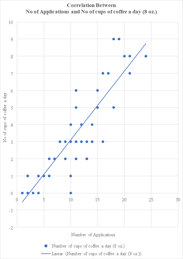 Scatter Diagram:
In the scatter diagram it is shown, the value of the independent variable (number of applications) along the X-axis and the value of the dependent (number of cups of coffee a day) on the Y-axis. For each pair of X and Y values (Xi, Yi), I plotted dots on graph paper for the pairs of observation. The diagram of dots obtained is called scatter diagram.
From the scatter diagram we can know the direction of correlation (positive or negative) but we cannot know the degree of correlation (numerical value of correlation) between the two variables. By looking to the scatter of the various points, we can get an idea whether the variables are related or not.
Discussion/ Validity:
The Pearson correlation coefficient measures the strength of the linear relation between two variables. It can be used to estimate the population correlation, ρ.
This graph shows that there is highly positive correlation between number of applications and number of cups of coffee a day (8 oz.) among high school students.
Limitations:
There are some limitations of this research project which may lead to wrong conclusions:
Correlation are always based on available data and it does not allow me to go beyond this data. There are number of factors other than number of applications and (Independent Variable) which may influence on number of cups of coffee a day (8 oz.) (Dependent Variable) of the students– such as stress, socio economic conditions, relation with friends and family members etc.
To establish relation between two variables it is assumed that there is linear relationship between them, whether such kind of relationship may exist or not. Some of the observations affect the value of coefficient of correlation and may provide misleading information. Finally, if there is a strong correlation between two variables it does not imply there is a cause and effect relationship between them. In this case, other factors can influence this relationship.
Conclusion:
On the basis of the statistical data and mathematical calculations, there is a high degree of positive correlation between number of applications and number of cups of coffee a day (8 oz.). The number of college students who suffer from stress-related problems appears to be on the rise.
Occasional stress is an unavoidable part of our routine life. Small amounts of stress can even have a positive effect on students, allowing us to push themselves when they encountered a difficult task. However, high levels of stress on students over a prolonged period of time are linked to increased rates of depression, anxiety, cardiovascular disease, and other potentially health-threatening issues. This conclusion shows us how important it is to learn how to manage stress by students before they suffer any adverse effects. It may be useful to potentiate the rise of awareness in identification of potential stress risks, stress management techniques, and resources that should be available to all high school students. However, we should not forget there are other factors that may affect the relationship between these two variables.
Bibliography:
- Correlation. (n.d.). Retrieved January 5, 2019, from http://www.stat.yale.edu/Courses/1997-98/101/correl.htm
Leave a Reply